Understanding the Bias-Variance Tradeoff: A Comprehensive Guide

When building machine learning models, one critical challenge is finding the right balance between making the model too simple and making it too complex. This is where the Bias-Variance Tradeoff comes into play. In this blog, we'll break down what this tradeoff means, why it’s important, and how to visualize it using Python code.

What is the Bias-Variance Tradeoff?

1. Bias

Bias refers to the error caused by the model being overly simplistic and failing to capture the underlying patterns in the data. This is called underfitting.

• Example: Fitting a straight line to data that clearly follows a curve. The model makes assumptions that are too simplistic and fails to adapt to the complexity of the data.

2. Variance

Variance refers to the error caused by the model being overly sensitive to the training data, including the noise. This is called overfitting.

• Example: Fitting a highly complex curve that not only captures the real pattern in the data but also fits random fluctuations (noise). The model becomes so specific to the training data that it performs poorly on new data.

3. The Tradeoff

The bias-variance tradeoff arises because as we try to decrease bias (make the model more complex), variance tends to increase. Conversely, as we reduce variance (simplify the model), bias increases.

The goal is to find the sweet spot where both bias and variance are balanced, resulting in a model that generalizes well to new, unseen data.

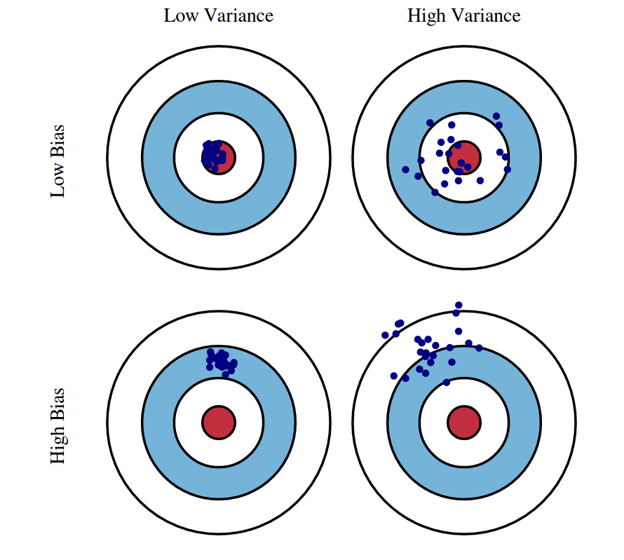
Visualizing the Concept

Let’s use an analogy to understand this intuitively:

• High Bias: Imagine throwing darts at a dartboard, but they all land far from the bullseye in the same spot. The model is consistent but wrong, as it fails to capture important patterns.
• High Variance: Now imagine the darts are scattered all over the dartboard, some near the bullseye and others far away. The model is too complex and inconsistent.
• Balanced: Ideally, we want the darts to land consistently close to the bullseye. This represents a model that has just the right balance between bias and variance.

A Practical Example with Python

Here’s a Python script to demonstrate underfitting, overfitting, and the balance point using synthetic data:

import numpy as np
import matplotlib.pyplot as plt
from sklearn.model_selection import train_test_split
from sklearn.preprocessing import PolynomialFeatures
from sklearn.linear_model import LinearRegression
from sklearn.metrics import mean_squared_error

# Generate synthetic data
np.random.seed(42)
X = np.random.rand(100, 1) * 10  # Random values between 0 and 10
y = 3 * X**2 + 2 * X + np.random.randn(100, 1) * 10  # Quadratic relationship with noise

# Split the data
X_train, X_test, y_train, y_test = train_test_split(X, y, test_size=0.2, random_state=42)

# Visualize data
plt.scatter(X, y, alpha=0.6, label='Data')
plt.xlabel("X")
plt.ylabel("y")
plt.title("Synthetic Data")
plt.legend()
plt.show()

# Fit models with increasing complexity
degrees = [1, 3, 15]  # Underfit, Good fit, Overfit
plt.figure(figsize=(15, 5))

for i, degree in enumerate(degrees):
    poly_features = PolynomialFeatures(degree=degree, include_bias=False)
    X_train_poly = poly_features.fit_transform(X_train)
    X_test_poly = poly_features.transform(X_test)
    
    model = LinearRegression()
    model.fit(X_train_poly, y_train)
    
    # Predictions
    X_plot = np.linspace(0, 10, 100).reshape(100, 1)
    X_plot_poly = poly_features.transform(X_plot)
    y_plot = model.predict(X_plot_poly)
    
    # Plot
    plt.subplot(1, 3, i + 1)
    plt.scatter(X_train, y_train, alpha=0.6, label='Train Data')
    plt.scatter(X_test, y_test, alpha=0.6, label='Test Data', color='r')
    plt.plot(X_plot, y_plot, label=f'Degree {degree} Fit', color='black')
    plt.title(f"Degree {degree} Fit")
    plt.xlabel("X")
    plt.ylabel("y")
    plt.legend()

plt.tight_layout()
plt.show()

# Evaluate models
for degree in degrees:
    poly_features = PolynomialFeatures(degree=degree, include_bias=False)
    X_train_poly = poly_features.fit_transform(X_train)
    X_test_poly = poly_features.transform(X_test)
    
    model = LinearRegression()
    model.fit(X_train_poly, y_train)
    
    train_mse = mean_squared_error(y_train, model.predict(X_train_poly))
    test_mse = mean_squared_error(y_test, model.predict(X_test_poly))
    print(f"Degree {degree}: Train MSE = {train_mse:.2f}, Test MSE = {test_mse:.2f}")

Explanation of the Code

• We create a synthetic quadratic dataset with noise to simulate real-world data.
• Models with increasing complexity (polynomial degrees 1, 3, and 15) are trained and visualized.
• The performance of each model is evaluated using the Mean Squared Error (MSE) for both training and test sets:
  • Degree 1 (Underfitting): The model is too simple and misses important patterns.
  • Degree 15 (Overfitting): The model is overly complex and captures noise.
  • Degree 3 (Balanced): The model achieves a good balance between bias and variance.

Key Takeaways

• Bias: The error from making overly simplistic assumptions.
• Variance: The error from being too sensitive to training data noise.
• The Tradeoff: Balancing bias and variance is critical for building a model that generalizes well.

Understanding the bias-variance tradeoff is an essential skill for any machine learning practitioner. It ensures your models perform consistently and accurately on new data.

Further Learning

If you enjoyed this blog, check out these resources:

1. Master Explainable AI with SHAP: Solving Kaggle's House Prices Dataset
2. Solving Kaggle’s Spaceship Titanic: Complete Walkthrough for Hyperparameter Optimization with Optuna

Stay tuned for more insights into machine learning fundamentals!