Time Series Forecasting - Part 1

Time series forecasting plays a crucial role in various domains, enabling us to predict future values based on historical data. In this article, we will embark on a journey into the world of time series forecasting, focusing on two fundamental concepts: the Hodrick-Prescott filter and ETS decomposition. Along the way, we will also explore the essential components of time series data, including trends, seasonality, and cyclic patterns. By leveraging the power of libraries such as Statsmodels, Pandas, Numpy, and Plotly, we will illustrate code examples to solidify our understanding. To accompany this article, you can find the corresponding Jupyter Notebook and tutorial video on GitHub and YouTube, respectively.

Introduction

Time series forecasting has gained significant importance in various industries and disciplines. Whether it's predicting stock prices, weather patterns, or customer demand, understanding and analyzing time series data is essential for making informed decisions. In this article, we will delve into the mathematical concepts and techniques behind time series forecasting, starting with the Hodrick-Prescott filter and ETS decomposition.

Components of Time Series Data

Before exploring advanced techniques, it's crucial to understand the components that makeup time series data. We will explore three fundamental components.

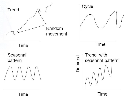
Trends

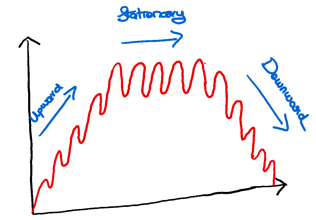
Trends represent the long-term movement or behavior of a time series. They can be upward (increasing), downward (decreasing), or even flat (no significant change). By identifying and analyzing trends, we can gain insights into the underlying patterns of the data.

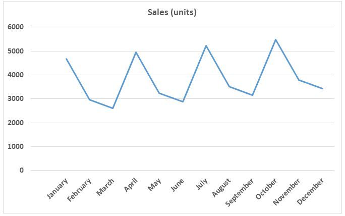
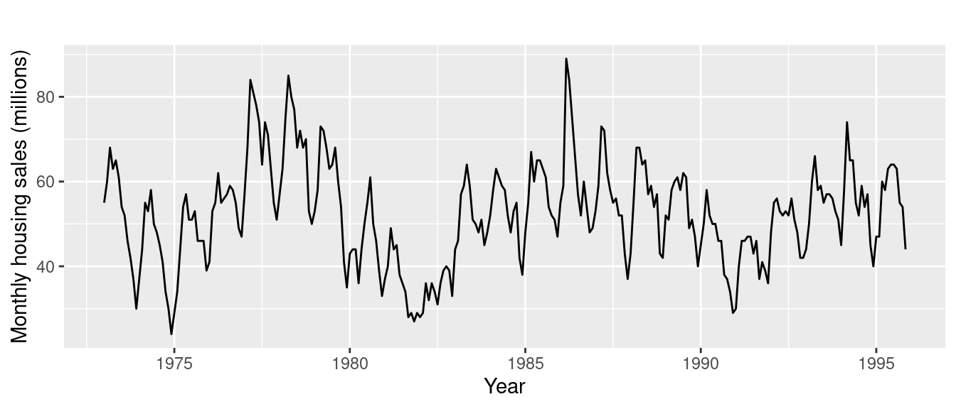
Seasonality

Seasonality refers to regular and predictable patterns that occur within a specific time frame. These patterns often repeat over fixed intervals, such as daily, weekly, monthly, or yearly. Understanding seasonality helps us identify and account for cyclical patterns in the data.

Cyclical

Cyclic components are similar to seasonality but do not have fixed and predictable intervals. They represent fluctuations or oscillations that occur over extended periods, usually more than a year. Unlike seasonality, cycles are not recurring at fixed intervals.

Hodrick-Prescott Filter

The Hodrick-Prescott filter is a popular technique used to decompose a time series into two components: trend and cyclical components. It separates the trend, which represents the long-term behavior, from the cyclical component, which captures short-term oscillations around the trend. This filter helps us understand the underlying structure of the time series and can be useful for forecasting.

The Hodrick-Prescott Filter separates a time-series \(y_t\) into a trend component \(\tau_t\) and a cyclical component \(c_t\) .

\[y_t = \tau_t + c_t\]

The trend and cyclical components are determined by minimizing the following quadratic loss function, where \(\lambda\) is the smoothing parameter.

\[min_{\tau_t} \sum_{t=1}^{T} {c_t}^2 + \lambda \sum_{t=1}^{T} [(\tau_t - \tau_{t-1}) - (\tau_{t-1} - \tau_{t-2})]^2\]

The \(\lambda\) value above handles variations in the growth rate of the trend component.

The ideal values of \(\lambda\) have already been identified,

• Default Data - 1600 (Recommended)
• Annual Data - 6.25
• Monthly Data - 129,600

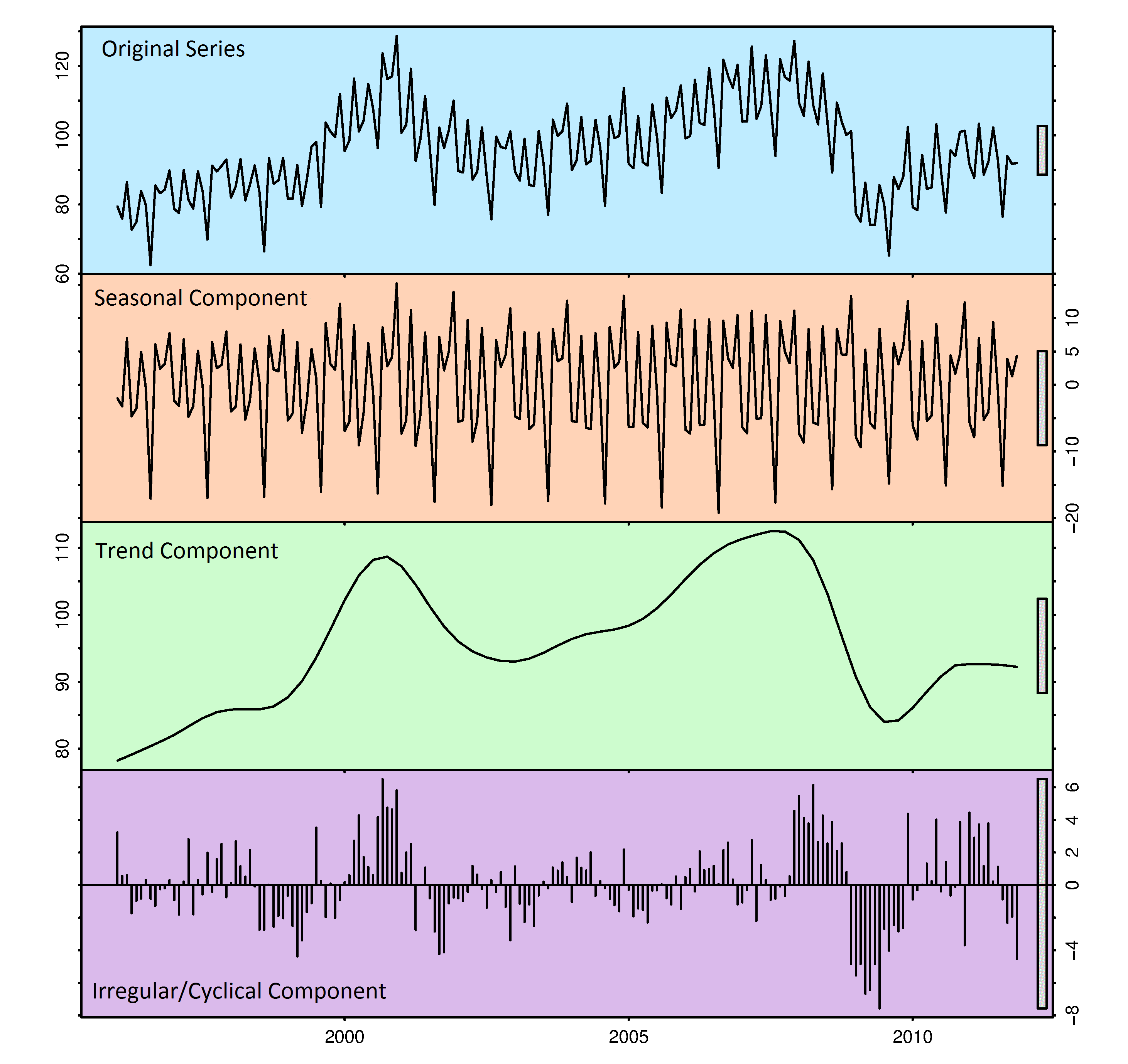
ETS Decomposition

ETS (Error, Trend, and Seasonality) decomposition is another powerful method for decomposing time series data. It breaks down the time series into three components: error, trend, and seasonality. The error component captures random fluctuations, the trend component represents long-term behavior, and the seasonality component accounts for regular and predictable patterns. ETS decomposition is widely used for analyzing and forecasting time series data. The Hodrick-Prescott Filter explored above can be seen as a simplistic version of ETS Decomposition.

There are two types of main ETS Models,

• Additive Model - Use when the Trend is more Linear, Seasonality, and Trend Components seem constant over time.
• Multiplicative Model - Use when the Trend increases or decreases at a non-linear rate.

Code Examples

In this section, we will demonstrate practical implementations of the concepts discussed using Python and several popular libraries.

Importing Necessary Libraries

We will start by importing the required libraries, including Statsmodels, Pandas, Numpy, and Plotly. These libraries provide powerful tools for time series analysis, data manipulation, numerical computations, and interactive visualizations.

%pip install pandas numpy plotly statsmodels --quiet

import pandas as pd
import numpy as np
from statsmodels.tsa.filters.hp_filter import hpfilter
from statsmodels.tsa.seasonal import seasonal_decompose
import plotly.express as px
from plotly.subplots import make_subplots

Loading Time Series Data

Next, we will load a time series dataset into our Jupyter Notebook. We can use Pandas, a versatile library for data manipulation, to load the data from a CSV file or any other compatible format.

# Read in data
gdp = pd.read_csv("https://github.com/LOST-STATS/lost-stats.github.io/raw/source/Time_Series/Data/GDPC1.csv")

# Convert date column to be of data type datetime64
gdp['DATE'] = pd.to_datetime(gdp['DATE'])

# Set the DATE as the index
gdp.set_index('DATE', inplace=True)

Now lets visualize the time series data,

# Plot the GDP Trends
fig = px.line(x=gdp.index, y=gdp['GDPC1'], title='Time Series', labels={'x':'Date', 'y':'GDP'})

# Display the Chart
fig.show()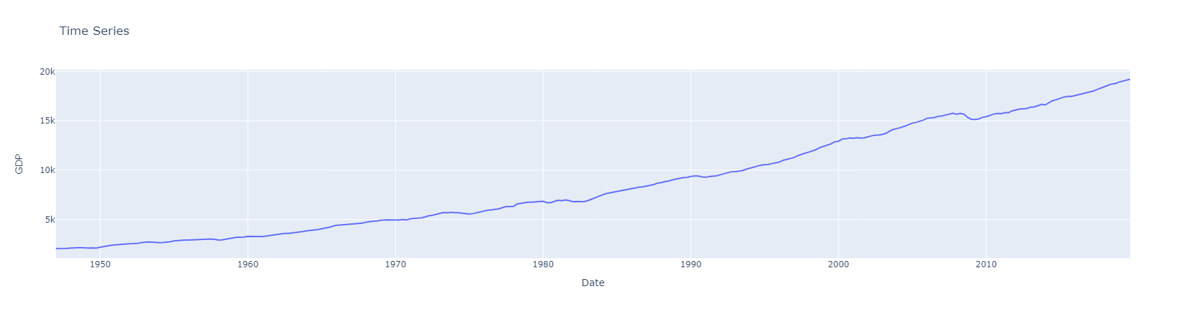

Applying the Hodrick-Prescott Filter:

To apply the Hodrick-Prescott filter, we will utilize the functionalities provided by the Statsmodels library. We will walk through the steps required to decompose the time series into its trend and cyclical components. By visualizing these components, we can gain insights into the long-term behavior and short-term oscillations of the data.

# Tuple Unpacking
# Lambda set to 1600 (Default) because data is quarterly
gdp_cycle, gdp_trend = hpfilter(gdp['GDPC1'], lamb=1600)

Visualizing the Cyclic and Trend components,

# Plot the Cyclical Component
fig = px.line(x=gdp_cycle.index, y=gdp_cycle, title='Cyclical Component', labels={'x':'Date', 'y':'Deviation'})

# Display the chart
fig.show()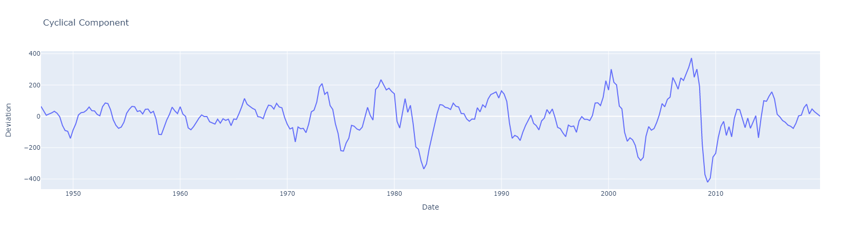

# Plot the Trend Component
fig = px.line(x=gdp_trend.index, y=gdp_trend, title='Trend Component', labels={'x':'Date', 'y':'GDP'})

# Display the Chart
fig.show()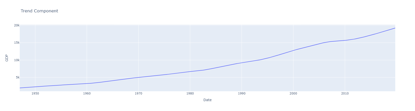

Performing ETS Decomposition:

Similar to the Hodrick-Prescott filter, we will use the Statsmodels library to perform ETS decomposition. We will showcase the process of decomposing the time series into error, trend, and seasonality components. By examining these components individually, we can better understand the patterns and fluctuations present in the data.

result = seasonal_decompose(gdp['GDPC1'], model='multiplicative')

We choose the multiplicative model due to the exponential increase observed in the trend as seen when visualizing the time series data.

# Create subplots with one row and four columns
fig = make_subplots(rows=4, cols=1, subplot_titles=['Original Time Series', 'Trend Component', 'Seasonal Component', 'Residual Component'])

# Add the original time series subplot
fig.add_trace(px.line(x=result.observed.index, y=result.observed, color_discrete_sequence=['black']).data[0], row=1, col=1)

# Add the trend component subplot
fig.add_trace(px.line(x=result.trend.index, y=result.trend, color_discrete_sequence=['blue']).data[0], row=2, col=1)

# Add the seasonal component subplot
fig.add_trace(px.line(x=result.seasonal.index, y=result.seasonal, color_discrete_sequence=['green']).data[0], row=3, col=1)

# Add the residual component subplot
fig.add_trace(px.line(x=result.resid.index, y=result.resid, color_discrete_sequence=['red']).data[0], row=4, col=1)

# Update layout
fig.update_layout(height=1000, title='ETS Decomposition Components', showlegend=False)

# Show the figure
fig.show()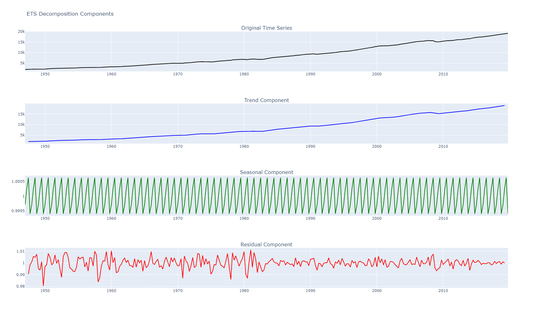

Conclusion

In this article, we explored the fundamental concepts and techniques of time series forecasting. We covered the essential components of time series data, including trends, seasonality, and cyclic components. Additionally, we dived into two popular decomposition methods: the Hodrick-Prescott filter and ETS decomposition.

To reinforce the concepts discussed, we provided code examples using Python and libraries such as Statsmodels, Pandas, Numpy, and Plotly. These examples demonstrated how to load and explore time series data, apply the Hodrick-Prescott filter, and perform ETS decomposition.

To access the accompanying resources, please find the following links:

• GitHub Repository: Access the Jupyter Notebook and code examples.
• Tutorial Video: Watch the tutorial video for a step-by-step explanation of the concepts covered in this article.

By mastering these fundamental concepts and techniques, you can enhance your ability to analyze and forecast time series data effectively. Time series forecasting is a powerful tool that can provide valuable insights and aid in decision-making across various domains.

Happy forecasting!