Stochastic Gradient Descent (SGD) with Momentum and Nesterov Accelerated Gradient

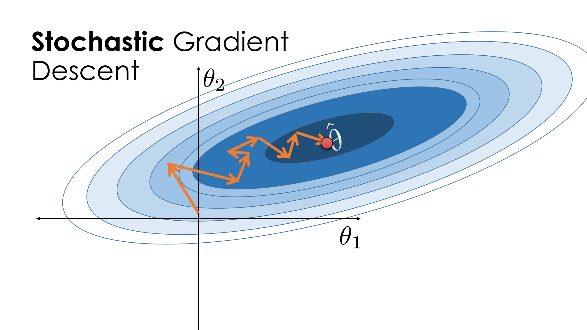
When training machine learning models, choosing the right optimizer can significantly impact the speed and efficiency of convergence. In this blog, we’ll explore two powerful upgrades to the classic Stochastic Gradient Descent (SGD): Momentum and Nesterov Accelerated Gradient (NAG). By the end, you'll have a clear understanding of their concepts, mathematics, and practical implementations.

Introduction to SGD

Stochastic Gradient Descent is the foundation of most optimization algorithms in machine learning. It works by iteratively updating the model's parameters in the direction of the negative gradient of the loss function.

Update Rule:
\(w = w - \eta \nabla L(w)\)

• ( \(w\) ): Model parameters (weights)
• ( \(\eta\) ): Learning rate
• ( \(\nabla L(w)\) ): Gradient of the loss function

However, SGD has limitations, such as:

1. Slow convergence in areas with flat gradients or ravines.
2. Sensitivity to noisy gradients, leading to oscillations.

To overcome these challenges, Momentum and NAG were introduced.

SGD with Momentum

Momentum enhances SGD by incorporating a "velocity" term, which helps the optimizer build up speed in consistent directions and dampen oscillations.

Key Intuition:
Imagine rolling a ball down a hill. It doesn’t stop immediately when the slope changes—it carries forward its velocity. Similarly, momentum helps the optimizer move faster in the right direction while smoothing oscillations.

Mathematics:

1. Velocity update:
   \(v_t = \beta v_{t-1} - \eta \nabla L(w)\)

Parameter update:
\(w = w + v_t\)

Here:

• ( \(\beta\) ): Momentum factor (usually 0.9)
• ( \(\eta\) ): Learning rate
• ( \(\nabla L(w)\) ): Gradient of the loss function

Benefits:

• Accelerates convergence, especially in flat regions of the loss landscape.
• Reduces oscillations in ravines where gradients differ sharply.

Nesterov Accelerated Gradient (NAG)

NAG improves on momentum by "looking ahead" at the future position of the parameters before computing the gradient.

Key Intuition:
While driving, anticipating a turn allows you to adjust the wheel in advance. NAG uses this concept by calculating the gradient at a "look-ahead" position.

Mathematics:

1. Look-ahead position:
   
   \(\tilde{w} = w + \beta v_{t-1}\)
2. Gradient calculation:
   
   \(g = \nabla L(\tilde{w})\)
3. Velocity update:
   
   \(v_t = \beta v_{t-1} - \eta g\)
4. Parameter update:
   
   \(w = w + v_t\)

Benefits:

• Provides a more precise update by considering future gradients.
• Further reduces oscillations and overshooting compared to momentum alone.

Code Implementation

Let’s see how to implement these optimizers in Python.

Vanilla SGD

# Dummy loss function
def gradient(x):
    return 2 * (x - 3)

x = 0  # Initial value
learning_rate = 0.1
iterations = 50

for _ in range(iterations):
    grad = gradient(x)
    x -= learning_rate * grad
    print(f"x: {x:.4f}")

SGD with Momentum

x = 0
velocity = 0
momentum = 0.9

for _ in range(iterations):
    grad = gradient(x)
    velocity = momentum * velocity - learning_rate * grad
    x += velocity
    print(f"x: {x:.4f}")

Nesterov Accelerated Gradient

x = 0
velocity = 0

for _ in range(iterations):
    look_ahead = x + momentum * velocity
    grad = gradient(look_ahead)
    velocity = momentum * velocity - learning_rate * grad
    x += velocity
    print(f"x: {x:.4f}")

Using PyTorch

import torch.optim as optim

# Example model
model = torch.nn.Linear(1, 1)

# SGD with Momentum
optimizer_momentum = optim.SGD(model.parameters(), lr=0.1, momentum=0.9)

# NAG
optimizer_nag = optim.SGD(model.parameters(), lr=0.1, momentum=0.9, nesterov=True)

Real-World Applications

1. Faster Convergence: Momentum and NAG significantly reduce the training time for machine learning models.
2. Smooth Optimization: Both methods handle noisy gradients and oscillations better, making them ideal for complex loss landscapes.
3. Widely Adopted: These optimizers are used in state-of-the-art deep learning frameworks like PyTorch and TensorFlow.

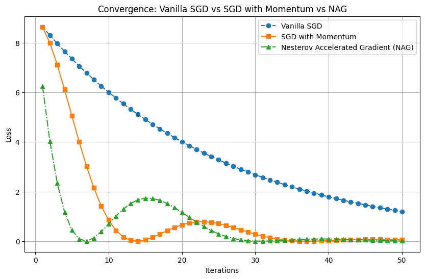
Comparison: Vanilla SGD, Momentum, and NAG

Below is a visualization showing the convergence speeds of the three methods.

Conclusion

Momentum and Nesterov Accelerated Gradient are essential tools in any machine learning practitioner’s toolkit. They are simple upgrades to SGD that make a big difference in training efficiency and model performance.